The sspse package
This is an R package to implement successive sampling population size estimation (SS-PSE).
SS-PSE is used to estimate the size of hidden populations using respondent-driven sampling (RDS) data. The package can implement SS-PSE, visibility SS-PSE, and capture-recapture SS-PSE.
The package was developed by the Hard-to-Reach Population Methods Research Group (HPMRG).
Installation
The package is available on CRAN and can be installed using
install.packages("sspse")
To install the latest development version from github, the best way it to use git to create a local copy and install it as usual from there. If you just want to install it, you can also use:
# If devtools is not installed:
# install.packages("devtools")

devtools::install_github("HPMRG/sspse")
Implementation
Load package and example data
library(sspse)
data(fauxmadrona)
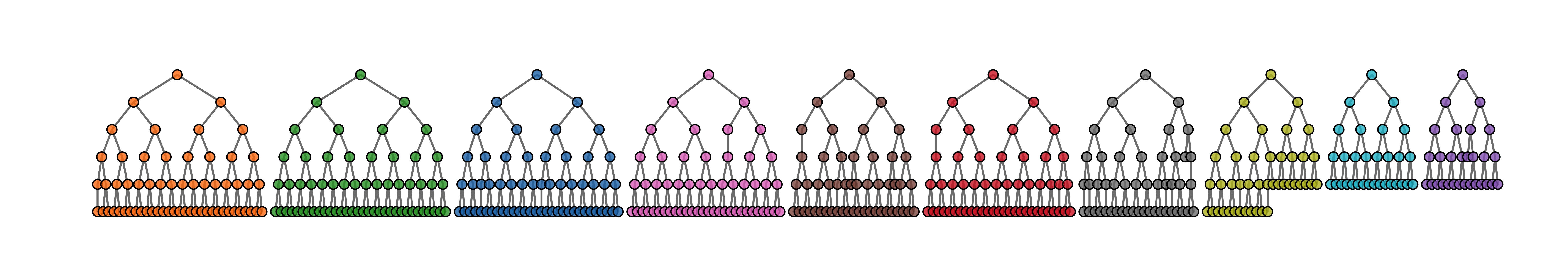
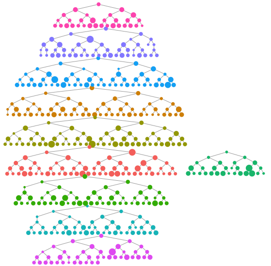
fauxmadrona is a simulated RDS data set with no seed dependency, which is used to demonstrate RDS estimators. It has the format of an rds.data.frame and is a sample of size 500 with 10 seeds and 2 coupons from a population of size 1000. For the purpose of this example, we will assume the population size is unknown and our goal is to estimate it.
We can make a quick visualization of the recruitment chains, where the size of the node is proportional to the reported degree and the color represents separate chains.
reingold.tilford.plot(fauxmadrona,
                      vertex.label=NA,
                      vertex.size="degree",
                      show.legend=FALSE,
                      vertex.color="seed")
The posteriorsize() function
The function that will perform both the original and visibility variants of SS-PSE is called posteriorsize(). It requires some prior knowledge
about the population size, $N$, which is usually expressed using the median.prior.size= argument.
Although there are many options within the posteriorsize function, most can be left at their default values unless you have a specific reason
to believe they should be set differently.
Original SS-PSE example
Set visibility=FALSE. By default, 1000 samples will be drawn from the posterior distribution for $N$ using a burnin of 1000 and an interval of
10. This may take a few seconds to run.
fit1 <- posteriorsize(fauxmadrona,
              median.prior.size=1000,
              visibility=FALSE)
## Using non-measurement error model with K = 14.
## Taken 1 samples...
## Taken 2 samples...
## Taken 4 samples...
...
## Taken 500 samples...
## Taken 1000 samples...
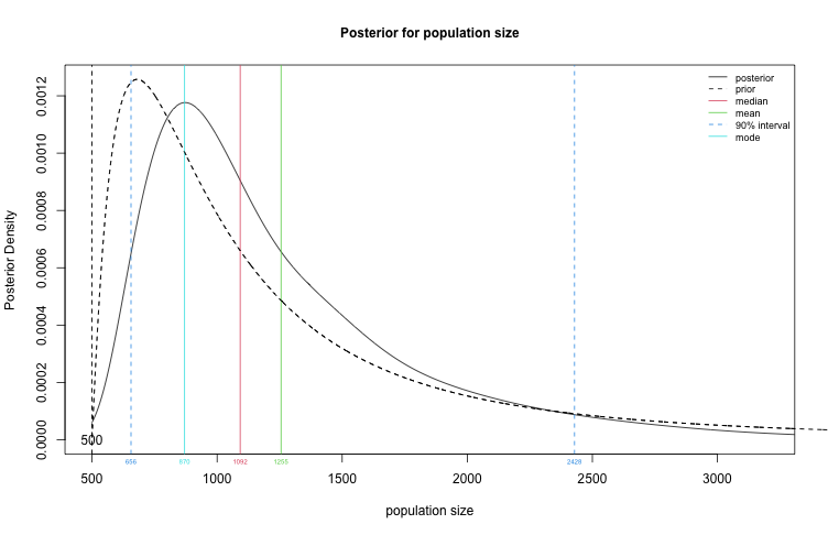
Plot the posterior distribution for $N$.
plot(fit1, type="N")
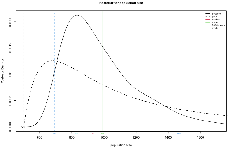
Create a table summary for the prior and posterior distributions for population size, specifying that we are interested in a 90% credible interval for $N$.
summary(fit1, HPD.level = 0.9)
## Summary of Population Size Estimation
##           Mean Median Mode 25%  75%  90%  5%  95%
## Prior     1247   1000  680 748 1480 2240 583 2852
## Posterior  974    936  874 808 1100 1275 656 1400
Example of Population Size Estimation Using Multiple Respondent-Driven Sampling Surveys
Suppose we have two respondent-driven sampling survey of the same population and taken successively in time. Then due to ideas in Kim and Handcock (2021) we can use the overlap between the respondents sampled in both surveys as additional information in estimating the population size. We mean additional information in the sense that it is in addition to the information in the two surveys ignoring the information in the overlap.
In this example, two samples are drawn from the fauxmadrona network. For the first survey, the sample size is 200.
For the second sample the sample size is 250. The second survey has an additional variable recapture
indicating if the respondent was also surveyed in the first survey.
First, let’s load the data:
data("fauxmadrona2")
The posteriorsize function can be used with both samples specified.
We estimate the posterior distribution for $N$ using a burnin of 1000 and an interval of
10. We set visibility=FALSE. This may take a few seconds to run.
crssfauxmadrona <- posteriorsize(fauxmadrona2[[1]], s2=fauxmadrona2[[2]], previous="recapture",
  visibility=FALSE,  median.prior.size=1250)
## Adjusting for the gross differences in the reported network sizes between the two samples.
## Using Capture-recapture non-measurement error model with K = 14.
## Taken 1 samples...
## Taken 2 samples...
## Taken 4 samples...
...
## Taken 500 samples...
## Taken 1000 samples...
Plot the posterior distribution for $N$.
plot(crssfauxmadrona, type="N")
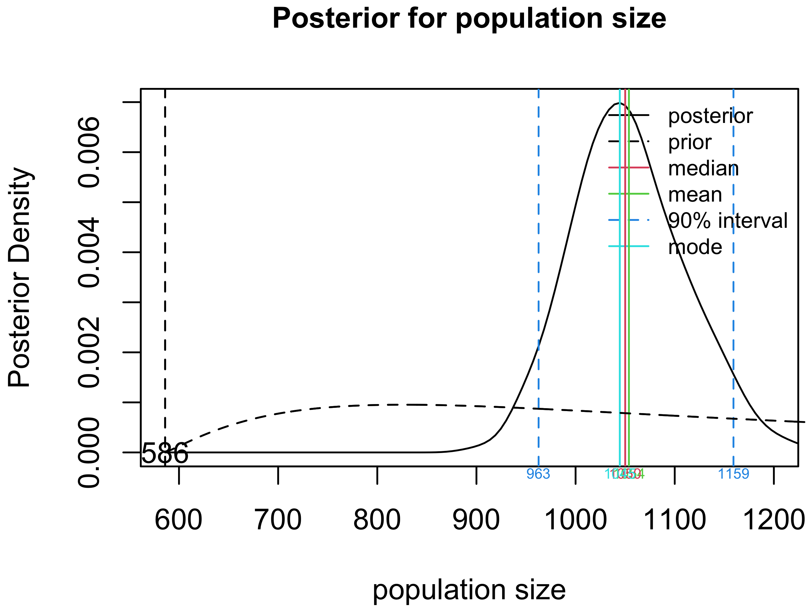
Create a table summary for the prior and posterior distributions for population size.
summary(crssfauxmadrona)
## Summary of Population Size Estimation
##           Mean Median Mode  25%  75%  90% 2.5% 97.5%
## Prior     1596   1250  826  918 1900 2953  662  4594
## Posterior 1055   1050 1039 1012 1094 1137  952  1170
Visibility SS-PSE example
Set visibility=TRUE. Because of the measurement error model, this model will take a little longer to fit - perhaps a minute or so.
fit2 <- posteriorsize(fauxmadrona,
              median.prior.size=1000,
              visibility=TRUE)
## Using a Exponentially Weighted Poisson measurement error model with K = 35.

## computing ...
## Taken 1 samples...
## Taken 2 samples...
...
## Taken 500 samples...
## Taken 1000 samples...
Summary of Population Size Estimation
Plot the posterior distribution for $N$.
plot(fit2, type="N")
Create a table summary for the prior and posterior distributions for population size, specifying that we are interested in a 90% credible interval for $N$.
summary(fit2, HPD.level = 0.9)
## Summary of Population Size Estimation
##           Mean Median Mode 25%  75%  90%  5%  95%
## Prior     1247   1000  680 748 1480 2240 583 2852
## Posterior 1275   1061  839 823 1486 2156 609 2732
Resources
Please use the GitHub repository to report bugs or request features: https://github.com/HPMRG/sspse
See the following papers for more information and examples:
Statistical Methodology
- Handcock, Mark S.; Gile, Krista J. and Mar, Corinne M. (2014) Estimating Hidden Population Size using Respondent-Driven Sampling Data, Electronic Journal of Statistics, 8(1):1491-1521.
- Handcock, Mark S.; Gile, Krista J. and Mar, Corinne M. (2015) Estimating the Size of Populations at High Risk for HIV using Respondent-Driven Sampling Data, Biometrics, 71(1):258-266.
- Kim, Brian J. and Handcock, Mark S. (2021) Population Size Estimation Using Multiple Respondent-Driven Sampling Surveys, Journal of Survey Statistics and Methodology, 9(1):94–120.
- McLaughlin, Katherine R.; Johnston, Lisa G.; Jakupi, Xhevat; Gexha-Bunjaku, Dafina; Deva, Edona and Handcock, Mark S. 2024 Modeling the Visibility Distribution for Respondent-Driven Sampling with Application to Population Size Estimation, The Annals of Applied Statistics, 18(1): 683-703 (March 2024).
Applications
- Johnston, Lisa G., McLaughlin, Katherine R., El Rhilani, Houssine, Latifi, Amina, Toufik, Abdalla, Bennani, Aziza, Alami, Kamal, Elomari, Boutaina, and Handcock, Mark S. (2015) Estimating the Size of Hidden Populations Using Respondent-driven Sampling Data: Case Examples from Morocco, Epidemiology, 26(6):846-852.
- Johnston, Lisa G., McLaughlin, Katherine R., Rouhani, Shada A., and Bartels, Susan A. (2017) Measuring a Hidden Population: A Novel Technique to Estimate the Population Size of Women with Sexual Violence-Related Pregnancies in South Kivu Province, Democratic Republic of Congo, Journal of Epidemiology and Global Health, 7(1):45-53.
- McLaughlin, Katherine R., Johnston, Lisa G., Gamble, Laura J., Grigoryan, Trdat, Papoyan, Arshak, and Grigoryan, Samvel (2019) Population Size Estimations Among Hidden Populations Using Respondent-Driven Sampling Surveys: Case Studies From Armenia, JMIR Public Health and Surveillance, 5(1):e12034.
- Johnston, Lisa G., McLaughlin, Katherine R., Gios, Lorenzo, Cordioli, Maddalena, Staneková, Danica V.,Blondeel, Karel, Toskin, Igor, Mirandola, Massimo, and The SIALON II Network (2021) Populations size estimations using SS-PSE among MSM in four European cities: how many MSM are living with HIV?, European Journal of Public Health, 31(6):1129–1136.